Chapter 9 Collaborating with GitHub
9.1 Overview
The collaborative power of GitHub and RStudio is really game changing. So far we’ve been collaborating with our most important collaborator: ourselves. But, we are lucky that in science we have so many other collaborators, so let’s learn how to use GitHub with one of them.
We are going to teach you the simplest way to collaborate with someone, which is for both of you to have administration privileges. GitHub is built for software developer teams, and there is a lot of features that we as scientists won’t use immediately.
We will do this all with a partner, and we’ll walk through some things all together, and then give you a chance to work with your collaborator on your own.
Objectives
- create a new repo and give permission to a collaborator
- open as a new RStudio project!
- collaborate with a partner
- explore github.com blame, history, issues
Resources
9.2 Create gh-pages repo
Team up with a partner sitting next to you. One of you will create a repository with a gh-pages branch from their computer. A reminder from Chapter 4: Create a repository on Github.com.
9.3 Give your collaborator administration priviledges
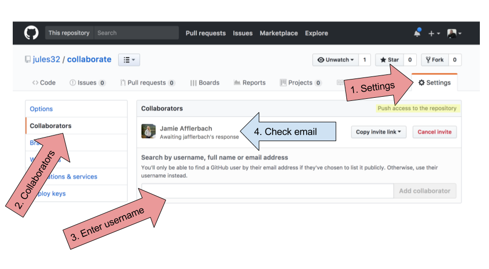
Now, go into Settings > Collaborators > enter your collaborator’s username.
Your collaborator then needs to check their email and accept as a collaborator. Notice that your collborator has “Push access to the repository” (highlighted below):
9.4 Clone to a new Rproject
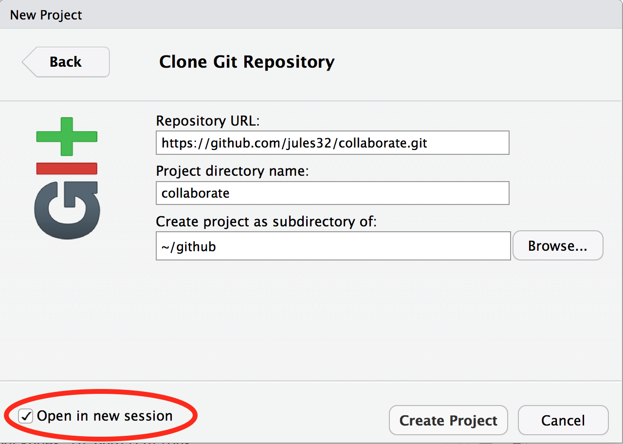
Once your collaborator accepts, you can both clone the repository to your local computer. We’ll do this through RStudio like we did before (see Chapter 4: Clone your repository using RStudio), but with a final additional step before hitting “Create Project”: select “Open in a new Session”.
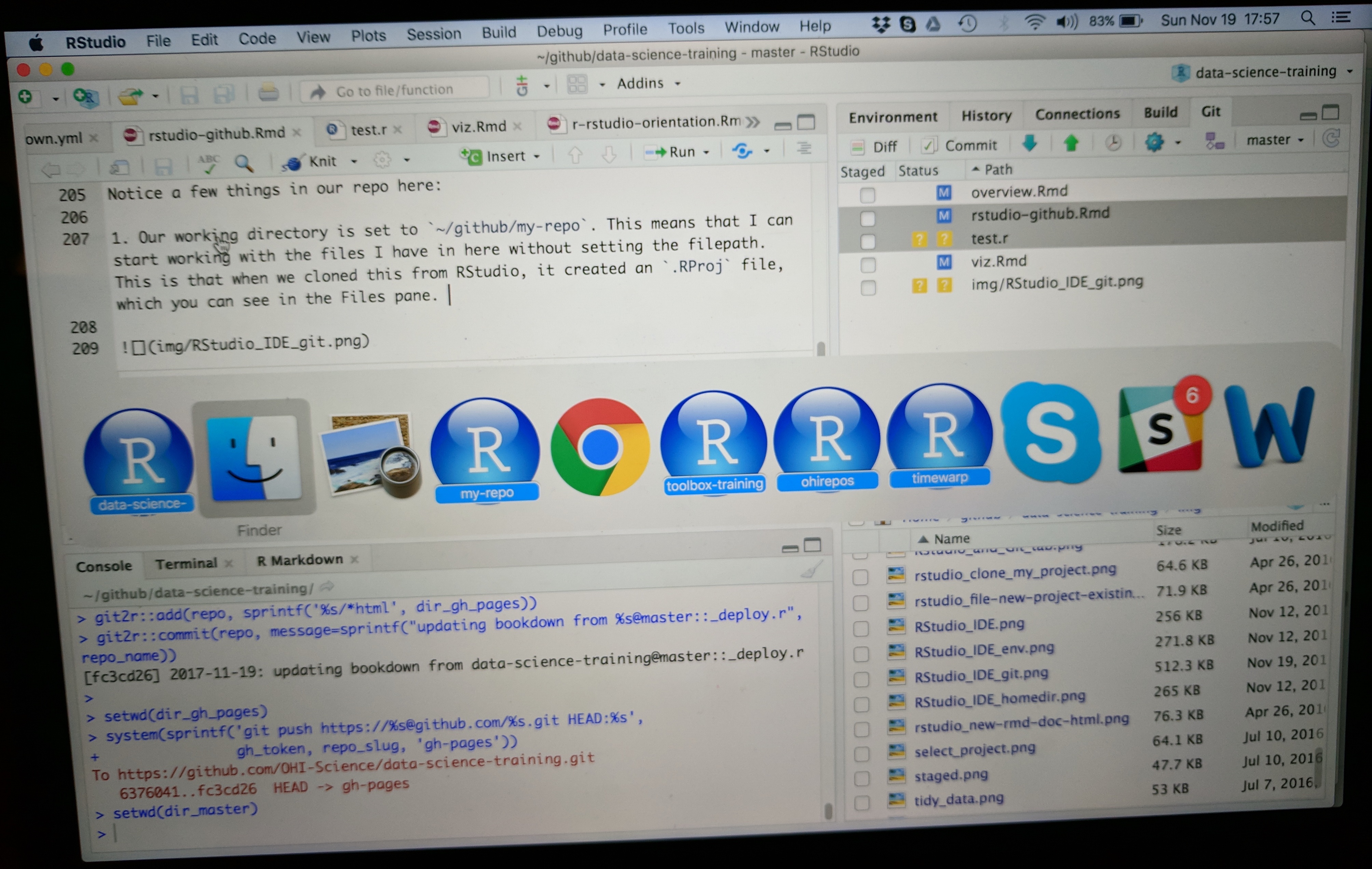
Opening this Project in a new Session opens up a new world of awesomeness from RStudio. Having different RStudio project sessions allows you to keep your work separate and organized. So you can collaborate with your collaborator on this repository while also working on your other repository from this morning. I tend to have a lot of projects going at one time:
9.5 Collaborative analysis
Now that you both have the same repo cloned to your computers, let’s start collaborating. We’ll be playing around with airline flights data, so let’s get setup a bit.
- Person 1: update the README to say something about you two, the authors.
- Person 2: create an RMarkdown file, add something about the authors, and knit it.
- Both of you: sync to GitHub.com (pull, stage, commit, push).
- Both of you: once you’ve both synced (talk to each other about it!), pull again. You should see each others’ work on your computer.
- Person 1: in the RMarkdown file, add a bit of the plan. We’ll be exploring the
nycflights13dataset. This is data on flights departing New York City in 2013. - Person 2: in the README, add a bit of the plan.
- Both of you: sync
9.6 Explore on GitHub.com
Now, let’s look at the repo again on GitHub.com. You’ll see those new files appear, and the commit history has increased.
9.6.1 Commit History
You’ll see that the number of commits for the repo has increased, let’s have a look. You can see the history of both of you.
9.6.2 Blame
Now let’s look at a single file, starting with the README file. We’ve explored the “Raw” and “History” options in the top-right of the file, but we haven’t really explored the “Blame” option. Let’s look now. Blame shows you line-by-line who authored the most recent version of the file you see. This is super useful if you’re trying to understand logic; you know who to ask for questions or attribute credit.
9.6.3 Issues
Now let’s have a look at issues. This is a way you can communicate to others about plans for the repo, questions, etc. Note that issues are public if the repository is public.
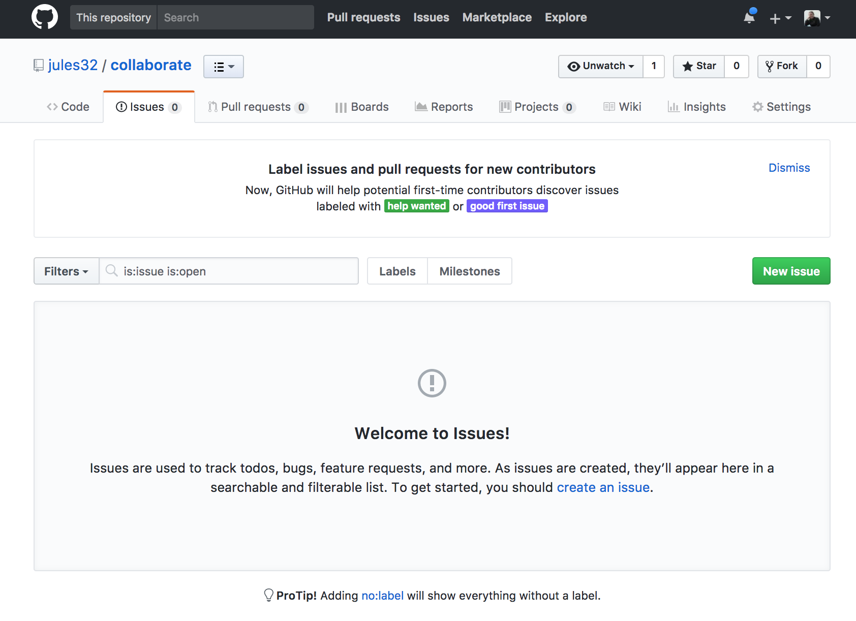
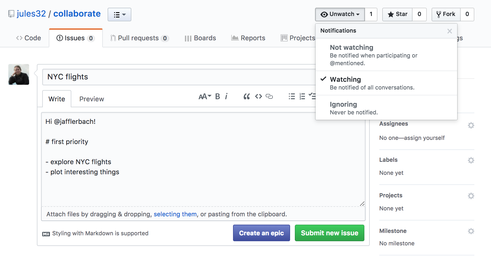
Let’s create a new issue with the title “NYC flights”.
In the text box, let’s write a note to our collaborator. You can use Markdown in this text box, which means all of your header and bullet formatting will come through. You can also select these options by clicking them just above the text box.
Let’s have one of you write something here. I’m going to write:
Hi @jafflerbach!

# first priority

- explore NYC flights
- plot interesting things
Note that I have my collaborator’s GitHub name with a @ symbol. This is going to email her directly so that she sees this issue. I can click the “Preview” button at the top left of the text box to see how this will look rendered in Markdown. It looks good!
Now let’s click submit new issue.
On the right side, there are a bunch of options for categorizing and organizing your issues. You and your collaborator may want to make some labels and timelines, depending on the project.
Another feature about issues is whether you want any notifications to this repository. Click where it says “Unwatch” up at the top. You’ll see three options: “Not watching”, “Watching”, and “Ignoring”. By default, you are watching these issues because you are a collaborator to the repository. But if you stop being a big contributor to this project, you may want to switch to “Not watching”. Or, you may want to ask an outside person to watch the issues. Or you may want to watch another repo yourself!
Let’s have Person 2 respond to the issue affirming the plan.
9.7 NYC flights exploration
Let’s continue this workflow with your collaborator, syncing to GitHub often and practicing what we’ve learned so far. We will get started together and then you and your collaborator will work on your own.
Here’s what we’ll be doing (from R for Data Science’s Transform Chapter):
Data: You will be exploring a dataset on flights departing New York City in 2013. These data are actually in a package called nycflights13, so we can load them the way we would any other package.
Let’s have Person 1 write this in the RMarkdown document (Person 2 just listen for a moment; we will sync this to you in a moment).
library(nycflights13) # install.packages('nycflights13')
library(tidyverse)
This data frame contains all 336,776 flights that departed from New York City in 2013. The data comes from the US Bureau of Transportation Statistics, and is documented in ?flights.
flights## # A tibble: 336,776 x 19
## year month day dep_time sched_dep_time dep_delay arr_time
## <int> <int> <int> <int> <int> <dbl> <int>
## 1 2013 1 1 517 515 2 830
## 2 2013 1 1 533 529 4 850
## 3 2013 1 1 542 540 2 923
## 4 2013 1 1 544 545 -1 1004
## 5 2013 1 1 554 600 -6 812
## 6 2013 1 1 554 558 -4 740
## 7 2013 1 1 555 600 -5 913
## 8 2013 1 1 557 600 -3 709
## 9 2013 1 1 557 600 -3 838
## 10 2013 1 1 558 600 -2 753
## # ... with 336,766 more rows, and 12 more variables: sched_arr_time <int>,
## # arr_delay <dbl>, carrier <chr>, flight <int>, tailnum <chr>,
## # origin <chr>, dest <chr>, air_time <dbl>, distance <dbl>, hour <dbl>,
## # minute <dbl>, time_hour <dttm>Let’s select all flights on January 1st with:
filter(flights, month == 1, day == 1)## # A tibble: 842 x 19
## year month day dep_time sched_dep_time dep_delay arr_time
## <int> <int> <int> <int> <int> <dbl> <int>
## 1 2013 1 1 517 515 2 830
## 2 2013 1 1 533 529 4 850
## 3 2013 1 1 542 540 2 923
## 4 2013 1 1 544 545 -1 1004
## 5 2013 1 1 554 600 -6 812
## 6 2013 1 1 554 558 -4 740
## 7 2013 1 1 555 600 -5 913
## 8 2013 1 1 557 600 -3 709
## 9 2013 1 1 557 600 -3 838
## 10 2013 1 1 558 600 -2 753
## # ... with 832 more rows, and 12 more variables: sched_arr_time <int>,
## # arr_delay <dbl>, carrier <chr>, flight <int>, tailnum <chr>,
## # origin <chr>, dest <chr>, air_time <dbl>, distance <dbl>, hour <dbl>,
## # minute <dbl>, time_hour <dttm>To use filtering effectively, you have to know how to select the observations that you want using the comparison operators. R provides the standard suite: >, >=, <, <=, != (not equal), and == (equal). We learned these operations yesterday. But there are a few others to learn as well.
9.7.0.1 Sync
Sync this RMarkdown back to GitHub so that your collaborator has access to all these notes. Person 2 should then pull and will continue with the following notes:
9.7.1 Logical operators
Multiple arguments to filter() are combined with “and”: every expression must be true in order for a row to be included in the output. For other types of combinations, you’ll need to use Boolean operators yourself:
&is “and”|is “or”!is “not”
Let’s have a look:
The following code finds all flights that departed in November or December:
filter(flights, month == 11 | month == 12)The order of operations doesn’t work like English. You can’t write filter(flights, month == 11 | 12), which you might literally translate into “finds all flights that departed in November or December”. Instead it finds all months that equal 11 | 12, an expression that evaluates to TRUE. In a numeric context (like here), TRUE becomes one, so this finds all flights in January, not November or December. This is quite confusing!
A useful short-hand for this problem is x %in% y. This will select every row where x is one of the values in y. We could use it to rewrite the code above:
nov_dec <- filter(flights, month %in% c(11, 12))Sometimes you can simplify complicated subsetting by remembering De Morgan’s law: !(x & y) is the same as !x | !y, and !(x | y) is the same as !x & !y. For example, if you wanted to find flights that weren’t delayed (on arrival or departure) by more than two hours, you could use either of the following two filters:
filter(flights, !(arr_delay > 120 | dep_delay > 120))
filter(flights, arr_delay <= 120, dep_delay <= 120)
Whenever you start using complicated, multipart expressions in filter(), consider making them explicit variables instead. That makes it much easier to check your work.
9.8 Your turn
OK: Person 2, sync this to GitHub, and Person 1 will pull so that we all have the most current information.
With your partner, do the following tasks. Each of you should work on one task at a time. Since we’re working closely on the same document, talk to each other and have one person create a heading and a R chunk, and then sync; the other person can then create a heading and R chunk and sync, and then you can both work safely.
Remember to make your commit messages useful!
As you work, you may get merge conflicts. This is part of collaborating in GitHub; we will walk through and help you with these and also teach the whole group.
9.8.1 Use logicals
Find all flights that:
- Had an arrival delay of two or more hours
- Flew to Houston (
IAHorHOU) - Were operated by United, American, or Delta
- Departed in summer (July, August, and September)
- Arrived more than two hours late, but didn’t leave late
- Were delayed by at least an hour, but made up over 30 minutes in flight
- Departed between midnight and 6am (inclusive)
Another useful dplyr filtering helper is
between(). What does it do? Can you use it to simplify the code needed to answer the previous challenges?
9.8.2 Missing values
To answer these questions: read some background below.
How many flights have a missing
dep_time? What other variables are missing? What might these rows represent?Why is
NA ^ 0not missing? Why isNA | TRUEnot missing? Why isFALSE & NAnot missing? Can you figure out the general rule? (NA * 0is a tricky counterexample!)
One important feature of R that can make comparison tricky are missing values, or NAs (“not availables”). NA represents an unknown value so missing values are “contagious”: almost any operation involving an unknown value will also be unknown.
NA > 5## [1] NA10 == NA## [1] NANA + 10## [1] NANA / 2## [1] NAThe most confusing result is this one:
NA == NA## [1] NAIt’s easiest to understand why this is true with a bit more context:
# Let x be Mary's age. We don't know how old she is.
x <- NA

# Let y be John's age. We don't know how old he is.
y <- NA

# Are John and Mary the same age?
x == y
## [1] NA# We don't know!If you want to determine if a value is missing, use is.na():
is.na(x)## [1] TRUE