Chapter 3 R & RStudio, RMarkdown

3.1 Overview

Objectives

In this lesson we will:

• get oriented to the RStudio interface
• work with R in the console
• be introduced to built-in R functions
• learn to use the help pages
• explore RMarkdown
• configure git on our computers

Resources

This lesson is a combination of excellent lessons by others (thank you Jenny Bryan and Data Carpentry!) that I have combined and modified for our workshop today. I definitely recommend reading through the original lessons and using them as reference:

Dr. Jenny Bryan’s lectures from STAT545 at UBC

• R basics, workspace and working directory, RStudio projects
• Basic care and feeding of data in R

RStudio has great resources about its IDE (IDE stands for integrated development environment):

• webinars
• cheatsheets

3.2 Why learn R with RStudio

You are all here today to learn how to code. Coding made me a better scientist because I was able to think more clearly about analyses, and become more efficient in doing so. Data scientists are creating tools that make coding more intuitive for new coders like us, and there is a wealth of awesome instruction and resources available to learn more and get help.

Here is an analogy to start us off. If you were a pilot, R is an an airplane. You can use R to go places! With practice you’ll gain skills and confidence; you can fly further distances and get through tricky situations. You will become an awesome pilot and can fly your plane anywhere.

And if R were an airplane, RStudio is the airport. RStudio provides support! Runways, communication, community, and other services, and just makes your overall life easier. So it’s not just the infrastructure (the user interface or IDE), although it is a great way to learn and interact with your variables, files, and interact directly with GitHub. It’s also data science philosophy, R packages, community, and more. So although you can fly your plane without an airport and we could learn R without RStudio, that’s not what we’re going to do.

We are learning R together with RStudio and its many supporting features.

Something else to start us off is to mention that you are learning a new language here. It’s an ongoing process, it takes time, you’ll make mistakes, it can be frustrating, but it will be overwhelmingly awesome in the long run. We all speak at least one language; it’s a similar process, really. And no matter how fluent you are, you’ll always be learning, you’ll be trying things in new contexts, learning words that mean the same as others, etc, just like everybody else. And just like any form of communication, there will be miscommunications that can be frustrating, but hands down we are all better off because of it.

While language is a familiar concept, programming languages are in a different context from spoken languages, but you will get to know this context with time. For example: you have a concept that there is a first meal of the day, and there is a name for that: in English it’s “breakfast”. So if you’re learning Spanish, you could expect there is a word for this concept of a first meal. (And you’d be right: ‘desayuno’). We will get you to expect that programming languages also have words (called functions in R) for concepts as well. You’ll soon expect that there is a way to order values numerically. Or alphabetically. Or search for patterns in text. Or calculate the median. Or reorganize columns to rows. Or subset exactly what you want. We will get you increase your expectations and learn to ask and find what you’re looking for.

3.3 R at the console, RStudio goodies

Launch RStudio/R.

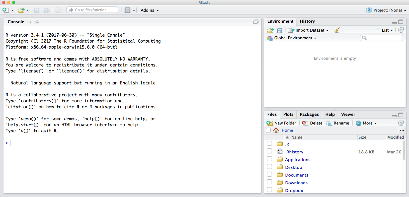
Notice the default panes:

• Console (entire left)
• Environment/History (tabbed in upper right)
• Files/Plots/Packages/Help (tabbed in lower right)

FYI: you can change the default location of the panes, among many other things: Customizing RStudio.

An important first question: where are we?

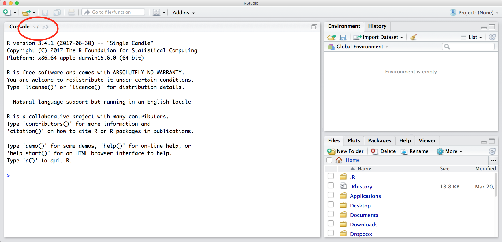
If you’ve just opened RStudio for the first time, you’ll be in your Home directory. This is noted by the ~/ at the top of the console. You can see too that the Files pane in the lower right shows what is in the Home directory where you are. You can navigate around within that Files pane and explore, but note that you won’t change where you are: even as you click through you’ll still be Home: ~/.

OK let’s go into the Console, where we interact with the live R process.

Make an assignment and then inspect the object you just created.

x <- 3 * 4
x

## [1] 12

In my head I hear, e.g., “x gets 12”.

All R statements where you create objects – “assignments” – have this form: objectName <- value.

I’ll write it in the command line with a hashtag #, which is the way R comments so it won’t be evaluated.

## objectName <- value

## This is also how you write notes in your code to explain what you are doing.

Object names cannot start with a digit and cannot contain certain other characters such as a comma or a space. You will be wise to adopt a convention for demarcating words in names.

# i_use_snake_case
# other.people.use.periods
# evenOthersUseCamelCase

Make an assignment

this_is_a_really_long_name <- 2.5

To inspect this variable, instead of typing it, we can press the up arrow key and call your command history, with the most recent commands first. Let’s do that, and then delete the assignment:

this_is_a_really_long_name

## [1] 2.5

Another way to inspect this variable is to begin typing this_…and RStudio will automagically have suggested completions for you that you can select by hitting the tab key, then press return.

One more:

science_rocks <- 100

Let’s try to inspect:

sciencerocks
# Error: object 'sciencerocks' not found

3.3.1 Error messages are your friends

Implicit contract with the computer / scripting language: Computer will do tedious computation for you. In return, you will be completely precise in your instructions. Typos matter. Case matters. Pay attention to how you type.

Remember that this is a language, not unsimilar to English! There are times you aren’t understood – it’s going to happen. There are different ways this can happen. Sometimes you’ll get an error. This is like someone saying ‘What?’ or ‘Pardon’? Error messages can also be more useful, like when they say ‘I didn’t understand this specific part of what you said, I was expecting something else’. That is a great type of error message. Error messages are your friend. Google them (copy-and-paste!) to figure out what they mean.

And also know that there are errors that can creep in more subtly, when you are giving information that is understood, but not in the way you meant. Like if I’m telling a story about tables and you’re picturing where you eat breakfast and I’m talking about data. This can leave me thinking I’ve gotten something across that the listener (or R) interpreted very differently. And as I continue telling my story you get more and more confused… So write clean code and check your work as you go to minimize these circumstances!

3.3.2 Logical operators and expressions

A moment about logical operators and expressions. We can ask questions about the objects we just made.

• == means ‘is equal to’
• != means ‘is not equal to’
• < means ` is less than’
• > means ` is greater than’
• <= means ` is less than or equal to’
• >= means ` is greater than or equal to’

science_rocks == 2

## [1] FALSE

science_rocks <= 30

## [1] FALSE

science_rocks != 5

## [1] TRUE

Shortcuts You will make lots of assignments and the operator <- is a pain to type. Don’t be lazy and use =, although it would work, because it will just sow confusion later. Instead, utilize RStudio’s keyboard shortcut: Alt + - (the minus sign). Notice that RStudio automagically surrounds <- with spaces, which demonstrates a useful code formatting practice. Code is miserable to read on a good day. Give your eyes a break and use spaces. RStudio offers many handy keyboard shortcuts. Also, Alt+Shift+K brings up a keyboard shortcut reference card.

My most common shortcuts include command-Z (undo), and combinations of arrow keys in combination with shift/option/command (moving quickly up, down, sideways, with or without highlighting.

When assigning a value to an object, R does not print anything. You can force R to print the value by using parentheses or by typing the object name:

weight_kg <- 55    # doesn't print anything
(weight_kg <- 55)  # but putting parenthesis around the call prints the value of `weight_kg`

## [1] 55

weight_kg          # and so does typing the name of the object

## [1] 55

Now that R has weight_kg in memory, we can do arithmetic with it. For instance, we may want to convert this weight into pounds (weight in pounds is 2.2 times the weight in kg):

2.2 * weight_kg

## [1] 121

We can also change a variable’s value by assigning it a new one:

weight_kg <- 57.5
2.2 * weight_kg

## [1] 126.5

This means that assigning a value to one variable does not change the values of other variables. For example, let’s store the animal’s weight in pounds in a new variable, weight_lb:

weight_lb <- 2.2 * weight_kg

and then change weight_kg to 100.

weight_kg <- 100

What do you think is the current content of the object weight_lb? 126.5 or 220? Why?

3.4 R functions, help pages

R has a mind-blowing collection of built-in functions that are used with the same syntax: function name with parentheses around what the function needs in order to do what it was built to do. When you type a function like this, we say we are “calling the function”. function_name(argument1 = value1, argument2 = value2, ...).

Let’s try using seq() which makes regular sequences of numbers and, while we’re at it, demo more helpful features of RStudio.

Type se and hit TAB. A pop up shows you possible completions. Specify seq() by typing more to disambiguate or using the up/down arrows to select. Notice the floating tool-tip-type help that pops up, reminding you of a function’s arguments. If you want even more help, press F1 as directed to get the full documentation in the help tab of the lower right pane.

Type the arguments 1, 10 and hit return.

seq(1, 10)

##  [1]  1  2  3  4  5  6  7  8  9 10

We could probably infer that the seq() function makes a sequence, but let’s learn for sure. Type (and you can autocomplete) and let’s explore the help page:

?seq 
help(seq) # same as ?seq

The help page tells the name of the package in the top left, and broken down into sections:

• Description: An extended description of what the function does.
• Usage: The arguments of the function and their default values.
• Arguments: An explanation of the data each argument is expecting.
• Details: Any important details to be aware of.
• Value: The data the function returns.
• See Also: Any related functions you might find useful.
• Examples: Some examples for how to use the function.

seq(from = 1, to = 10) # same as seq(1, 10); R assumes by position

##  [1]  1  2  3  4  5  6  7  8  9 10

seq(from = 1, to = 10, by = 2)

## [1] 1 3 5 7 9

The above also demonstrates something about how R resolves function arguments. You can always specify in name = value form. But if you do not, R attempts to resolve by position. So above, it is assumed that we want a sequence from = 1 that goes to = 10. Since we didn’t specify step size, the default value of by in the function definition is used, which ends up being 1 in this case. For functions I call often, I might use this resolve by position for the first argument or maybe the first two. After that, I always use name = value.

The examples from the help pages can be copy-pasted into the console for you to understand what’s going on. Remember we were talking about expecting there to be a function for something you want to do? Let’s try it.

3.4.1 Your turn

Exercise: Talk to your neighbor(s) and look up the help file for a function that you know or expect to exist. Here are some ideas: ?getwd(), ?plot(), min(), max(), ?mean(), ?log()).

And there’s also help for when you only sort of remember the function name: double-questionmark:

??install 

Not all functions have (or require) arguments:

date()

## [1] "Fri Dec  1 07:26:10 2017"

3.5 Clearing the environment

Now look at the objects in your environment (workspace) – in the upper right pane. The workspace is where user-defined objects accumulate.

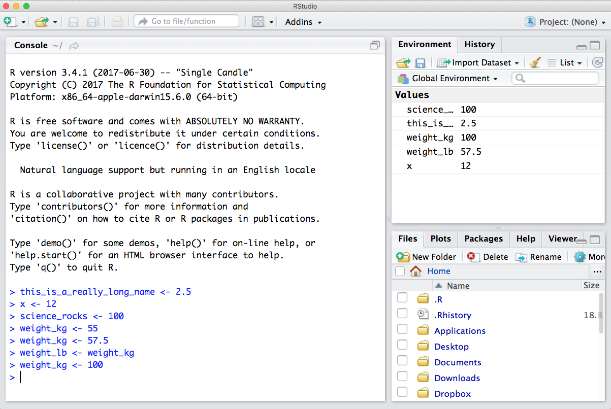
You can also get a listing of these objects with a few different R commands:

objects()

## [1] "science_rocks"              "this_is_a_really_long_name"
## [3] "weight_kg"                  "weight_lb"                 
## [5] "x"

ls()

## [1] "science_rocks"              "this_is_a_really_long_name"
## [3] "weight_kg"                  "weight_lb"                 
## [5] "x"

If you want to remove the object named weight_kg, you can do this:

rm(weight_kg)

To remove everything:

rm(list = ls())

or click the broom in RStudio’s Environment pane.

3.5.1 Your turn

Exercise: Clear your workspace, then create a few new variables. Create a variable that is the mean of a sequence of 1-20. What’s a good name for your variable? Does it matter what your ‘by’ argument is? Why?

3.6 RMarkdown

Now we are going to also introduce RMarkdown. This is really key for collaborative research, so we’re going to get started with it early and then use it for the rest of the day.

An Rmarkdown file will allow us to weave markdown text with chunks of R code to be evaluated and output content like tables and plots.

File -> New File -> Rmarkdown… -> Document of output format HTML, OK.

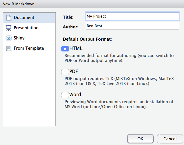
You can give it a Title like “My Project”. Then click OK.

OK, first off: by opening a file, we are seeing the 4th pane of the RStudio console, which is essentially a text editor. This lets us organize our files within RStudio instead of having a bunch of different windows open.

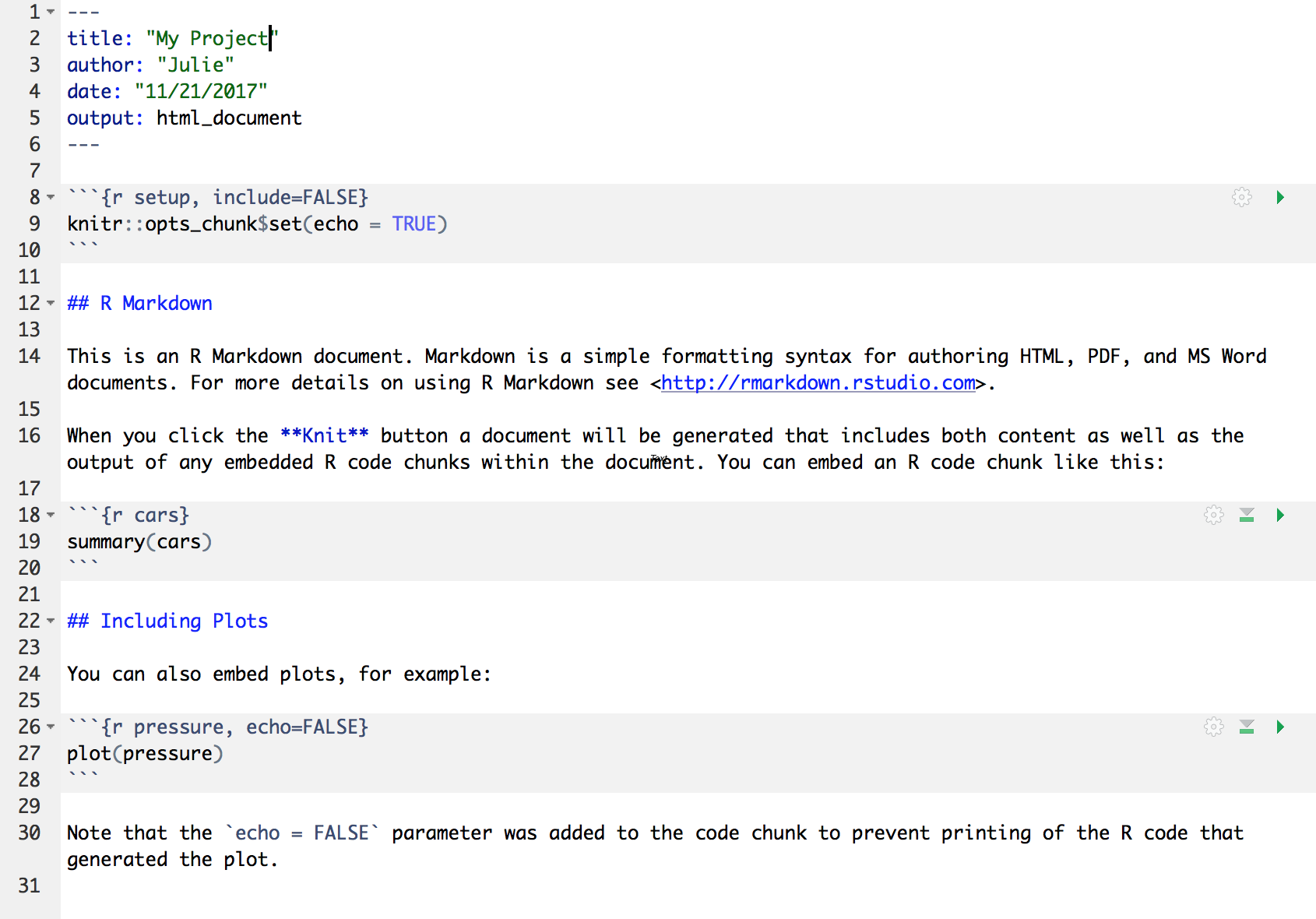
Let’s have a look at this file — it’s not blank; there is some initial text is already provided for you. Notice a few things about it:

• There are white and grey sections. R code is in grey sections, and other text is in white.

Let’s go ahead and “Knit HTML” by clicking the blue yarn at the top of the RMarkdown file.

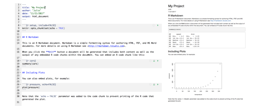
What do you notice between the two?

Notice how the grey R code chunks are surrounded by 3 backticks and {r LABEL}. These are evaluated and return the output text in the case of summary(cars) and the output plot in the case of plot(pressure).

Notice how the code plot(pressure) is not shown in the HTML output because of the R code chunk option echo=FALSE.

More details…

This RMarkdown file has 2 different languages within it: R and Markdown.

We don’t know that much R yet, but you can see that we are taking a summary of some data called ‘cars’, and then plotting. There’s a lot more to learn about R, and we’ll get into it for the next few days.

The second language is Markdown. This is a formatting language for plain text, and there are only about 15 rules to know.

Notice the syntax for:

• headers get rendered at multiple levels: #, ##
• bold: **word**

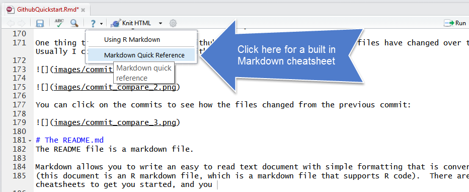
There are some good cheatsheets to get you started, and here is one built into RStudio:

Important: note that the hashtag # is used differently in Markdown and in R:

• in R, a hashtag indicates a comment that will not be evaluated. You can use as many as you want: # is equivalent to ######. It’s just a matter of style. I use two ## to indicate a comment so that it’s clearer what is a comment versus what I don’t want to run at the moment.
• in Markdown, a hashtag indicates a level of a header. And the number you use matters: # is a “level one header”, meaning the biggest font and the top of the hierarchy. ### is a level three header, and will show up nested below the # and ## headers.

Learn more: http://rmarkdown.rstudio.com/

3.6.1 Your Turn

1. In Markdown, Write some italic text, and make a numbered list. And add a few subheaders. Use the Markdown Quick Reference (in the menu bar: Help > Markdown Quick Reference).
2. Reknit your html file.

3.7 Troubleshooting

Here are some additional things we didn’t have time to discuss:

3.7.1 I just entered a command and nothing’s happening

It may be because you didn’t complete a command: is there a little + in your console? R is saying that it is waiting for you to finish. In the example below, I need to close that parenthesis.

> x <- seq(1, 10
+ 

3.7.2 How do I update RStudio?

To see if you have the most current version of RStudio, go to the Help bar > Check for Updates. If there is an update available, you’ll have the option to Quit and Download, which will take you to http://www.rstudio.com/download. When you download and install, choose to replace the previous version.