Chapter 7 Data Wrangling: `tidyr`

7.1 Overview

Now you have some experience wrangling and working with tidy data. But we all know that not all data that you have are tidy. So how do we make data more tidy? With the tidyr package.

Objectives

learn tidyr with the gapminder package
other wrangling: joins, binding
practice the RStudio-GitHub workflow
your turn: use the data wrangling cheat sheet to explore window functions

Resources

These materials borrow heavily from:

7.1.1 Setup

We’ll work today in RMarkdown. You can either continue from the same RMarkdown as yesterday, or begin a new one.

Here’s what to do:

Clear your workspace (Session > Restart R)
New File > R Markdown…, save as something other than gapminder-wrangle.Rmd and delete irrelevant info, or just continue using gapminder-wrangle.Rmd

I’m going to write this in my R Markdown file:

Data wrangling with `tidyr`, which is part of the tidyverse. We are going to tidy some data!

7.2 Finishing up dplyr

7.3 Joining datasets

Sometimes you have data coming from different places or in different files, and you want to put them together so you can analyze them. This is called relational data, because it has some kind of relationship. In the tidyverse, combining data that has a relationship is called “joining”.

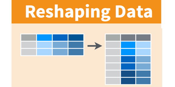
From the RStudio cheatsheet (note: this is an earlier version of the cheatsheet but I like the graphics):

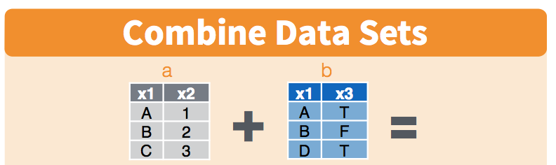
Notice how you may not have exactly the same observations in the x1 columns above. Observations A and B are the same, but notice how the table on the left has observation C, and the table on the right has observation D.

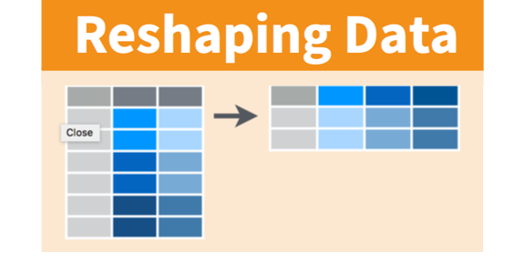
If you wanted to combine these two tables, how would you do it? There are some decisions you’d have to make about what was important to you. The cheatsheet visualizes it for us:

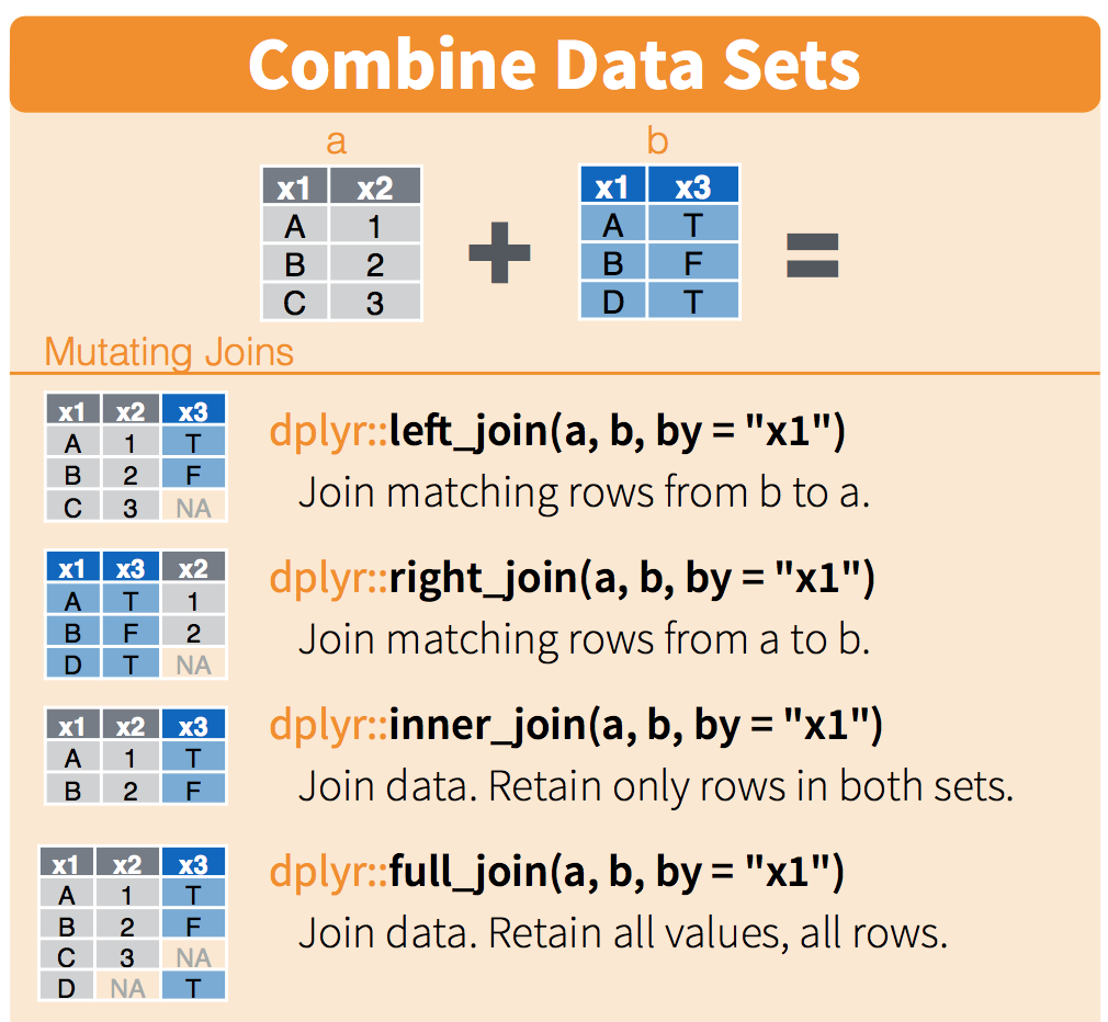
We will just talk about this briefly here, but you can refer to this more as you have your own datasets that you want to join. This describes the figure above::

left_join keeps everything from the left table and matches as much as it can from the right table. In R, the first thing that you type will be the left table (because it’s on the left)
right_join keeps everything from the right table and matches as much as it can from the left table
inner_join only keeps the observations that are similar between the two tables
full_join keeps all observations from both tables.

Let’s play with these CO2 emmissions data just to illustrate:

## read in the data. (same URL as yesterday, just with co2.csv instead of gapminder.csv)
co2 <- read_csv("https://raw.githubusercontent.com/OHI-Science/data-science-training/master/data/co2.csv")

## explore
co2 %>% head()
co2 %>% dim() # 12

## create new variable that is only 2007 data
gap_2007 <- gapminder %>%
  filter(year == 2007) 
gap_2007 %>% dim() # 142  

## left_join gap_2007 to co2
lj <- left_join(gap_2007, co2, by = "country")

## explore
lj %>% dim() #142
lj %>% summary() # lots of NAs in the co2_2017 columm
lj %>% View() 

## right_join gap_2007 and co2
rj <- right_join(gap_2007, co2, by = "country")

## explore
rj %>% dim() # 12
rj %>% summary()
rj %>% View()

That’s all we’re going to talk about today with joining, but there are more ways to think about and join your data. Check out the Relational Data Chapter in R for Data Science

7.3.1 load `tidyverse` (which has `tidyr` inside)

First load tidyr in an R chunk. You already have installed the tidyverse, so you should be able to just load it like this (using the comment so you can run install.packages("tidyverse") easily if need be):

library(tidyverse) # install.packages("tidyverse")

7.4 `tidyr` basics

Remember, from the dplyr section, that tidy data means all rows are an observation and all columns are variables.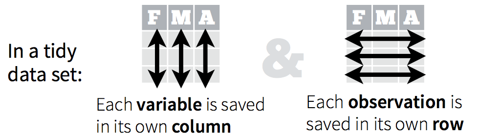

It’s important to recognize what shape your data is in, and work towards tidying it up.

Let’s take a look at some examples.

Data in the wide format each row is often a site/subject/patient and you have multiple observation variables containing the same type of data. These can be either repeated observations over time, or observation of multiple variables (or a mix of both). Data input may be simpler or some other applications may prefer the wide format. However, many of R’s functions have been designed assuming you have long format data.

A simple example of data in a wide format is the AirPassengers dataset which provides information on monthly airline passenger numbers from 1949-1960. You’ll notice that each row is a single year and the columns are each month Jan - Dec.

AirPassengers

##      Jan Feb Mar Apr May Jun Jul Aug Sep Oct Nov Dec
## 1949 112 118 132 129 121 135 148 148 136 119 104 118
## 1950 115 126 141 135 125 149 170 170 158 133 114 140
## 1951 145 150 178 163 172 178 199 199 184 162 146 166
## 1952 171 180 193 181 183 218 230 242 209 191 172 194
## 1953 196 196 236 235 229 243 264 272 237 211 180 201
## 1954 204 188 235 227 234 264 302 293 259 229 203 229
## 1955 242 233 267 269 270 315 364 347 312 274 237 278
## 1956 284 277 317 313 318 374 413 405 355 306 271 306
## 1957 315 301 356 348 355 422 465 467 404 347 305 336
## 1958 340 318 362 348 363 435 491 505 404 359 310 337
## 1959 360 342 406 396 420 472 548 559 463 407 362 405
## 1960 417 391 419 461 472 535 622 606 508 461 390 432

long format is the tidy data we are after, where:

each column is a variable
each row is an observation

In the long format, you usually have 1 column for the observed variable and the other columns are ID variables. The mpg dataset is an example of a long dataset with each row representing a single car and each column representing a variable of that car such as manufacturer and year.

mpg

## # A tibble: 234 x 11
##    manufacturer      model displ  year   cyl      trans   drv   cty   hwy
##           <chr>      <chr> <dbl> <int> <int>      <chr> <chr> <int> <int>
##  1         audi         a4   1.8  1999     4   auto(l5)     f    18    29
##  2         audi         a4   1.8  1999     4 manual(m5)     f    21    29
##  3         audi         a4   2.0  2008     4 manual(m6)     f    20    31
##  4         audi         a4   2.0  2008     4   auto(av)     f    21    30
##  5         audi         a4   2.8  1999     6   auto(l5)     f    16    26
##  6         audi         a4   2.8  1999     6 manual(m5)     f    18    26
##  7         audi         a4   3.1  2008     6   auto(av)     f    18    27
##  8         audi a4 quattro   1.8  1999     4 manual(m5)     4    18    26
##  9         audi a4 quattro   1.8  1999     4   auto(l5)     4    16    25
## 10         audi a4 quattro   2.0  2008     4 manual(m6)     4    20    28
## # ... with 224 more rows, and 2 more variables: fl <chr>, class <chr>

These different data formats mainly affect readability. For humans, the wide format is often more intuitive since we can often see more of the data on the screen due to it’s shape. However, the long format is more machine readable and is closer to the formatting of databases. The ID variables in our dataframes are similar to the fields in a database and observed variables are like the database values.

Note: Generally, mathematical operations are better in long format, although some plotting functions actually work better with wide format.

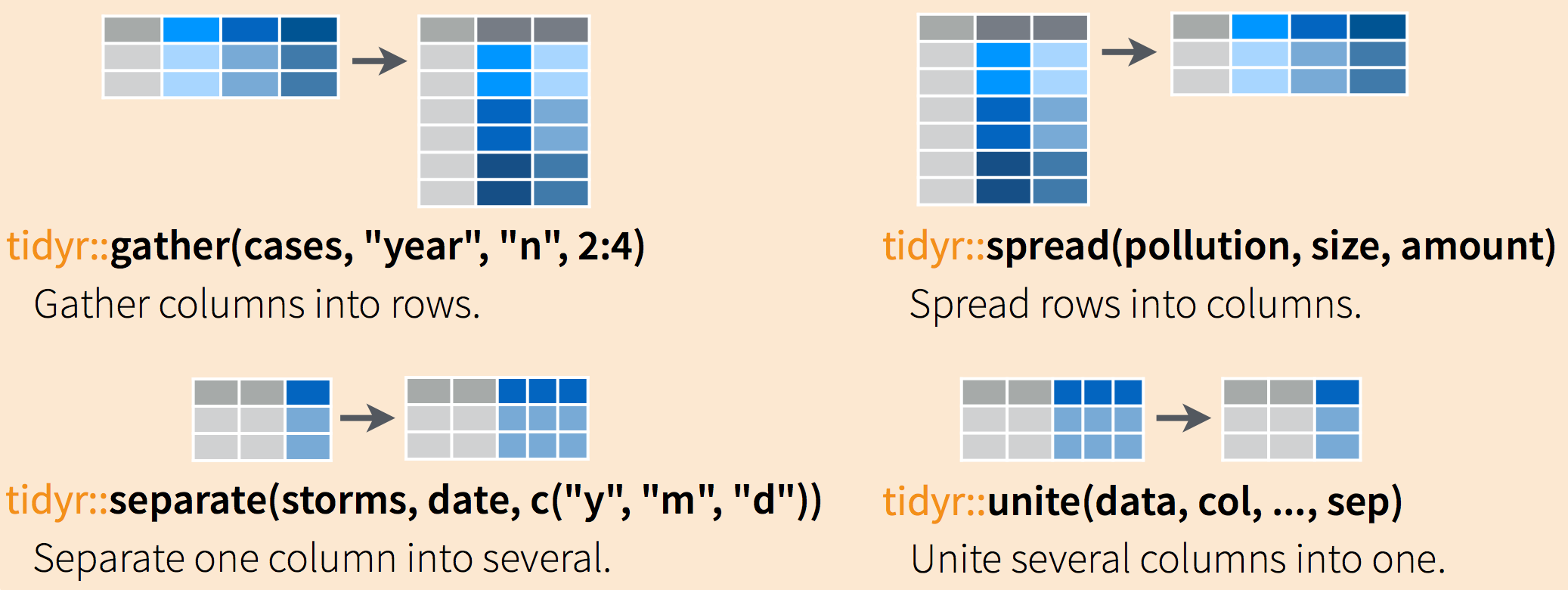
Often, data must be reshaped for it to become tidy data. What does that mean? There are four main verbs we’ll use, which are essentially pairs of opposites:

turn columns into rows (gather()),
turn rows into columns (spread()),
turn a character column into multiple columns (separate()),
turn multiple character columns into a single column (unite())

7.5 Explore gapminder dataset.

Yesterday we started off with the gapminder data in a format that was already tidy. But what if it weren’t? Let’s look at a different version of those data.

The data are on GitHub. Navigate there by going to:

github.com > ohi-science > data-science-training > data > gapminder_wide.csv

or by copy-pasting this in the browser: https://github.com/OHI-Science/data-science-training/blob/master/data/gapminder_wide.csv

Have a look at the data.

Question: Is gapminder a purely long, purely wide, or some intermediate format?

You can see there are a lot more columns than the version we looked at before. This format is pretty common, because it can be a lot more intuitive to enter data in this way.

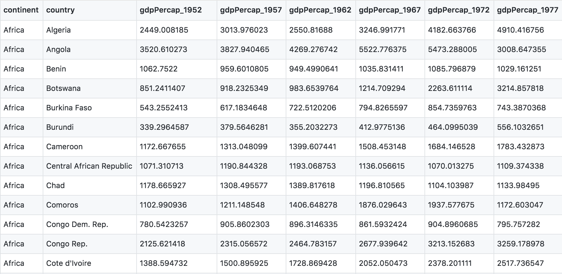
Sometimes, as with the gapminder dataset, we have multiple types of observed data. It is somewhere in between the purely ‘long’ and ‘wide’ data formats:

3 “ID variables” (continent, country, year)
3 “Observation variables” (pop,lifeExp,gdpPercap).

It’s pretty common to have data in this intermediate format in most cases despite not having ALL observations in 1 column, since all 3 observation variables have different units. But we can play with switching it to long format and wide to show what that means (i.e. long would be 4 ID variables and 1 observation variable).

But we want it to be in a tidy way so that we can work with it more easily. So here we go.

You use spread() and gather() to transform or reshape data between wide to long formats.

7.6 `gather()` data from wide to long format

Read in the data from GitHub. Remember, you need to click on the ‘Raw’ button first so you can read it directly. Let’s also read in the gapminder data from yesterday so that we can use it to compare later on.

## wide format
gap_wide <- readr::read_csv('https://raw.githubusercontent.com/OHI-Science/data-science-training/master/data/gapminder_wide.csv')

## yesterday's format (intermediate)
gapminder <- readr::read_csv('https://raw.githubusercontent.com/OHI-Science/data-science-training/master/data/gapminder.csv')

Let’s have a look:

head(gap_wide)
str(gap_wide)

While wide format is nice for data entry, it’s not nice for calculations. Some of the columns are a mix of variable (e.g. “gdpPercap”) and data (“1952”). What if you were asked for the mean population after 1990 in Algeria? Possible, but ugly. But we know it doesn’t need to be so ugly. Let’s tidy it back to the format we’ve been using.

Question: let’s talk this through together. If we’re trying to turn the gap_wide format into gapminder format, what structure does it have that we like? And what do we want to change?

We like the continent and country columns. We won’t want to change those.
For long format, we’d want just 1 column identifying the variable name (tidyr calls this a ‘key’), and 1 column for the data (tidyr calls this the ’value’).
For intermediate format, we’d want 3 columns for gdpPercap, lifeExp, and pop.
We would like year as a separate column.

Let’s get it to long format. We’ll have to do this in 2 steps. The first step is to take all of those column names (e.g. lifeExp_1970) and make them a variable in a new column, and transfer the values into another column. Let’s learn by doing:

Let’s have a look at gather()’s help:

?gather

Question: What is our key-value pair?

We need to name two new variables in the key-value pair, one for the key, one for the value. It can be hard to wrap your mind around this, so let’s give it a try. Let’s name them obstype_year and obs_values.

Here’s the start of what we’ll do:

gap_long <- gap_wide %>% 
  gather(key   = obstype_year,
         value = obs_values)

Although we were already planning to inspect our work, let’s definitely do it now:

str(gap_long)
head(gap_long)
tail(gap_long)

We have reshaped our dataframe but this new format isn’t necessarily what we wanted.

What went wrong? Notice that it didn’t know that we wanted to keep continent and country untouched; we need to give it more information about which columns we want reshaped. We can do this in several ways.

One way is to identify the columns is by name. Listing them explicitly can be a good approach if there are just a few. But in our case we have 30 columns. I’m not going to list them out here since there is way too much potential for error if I tried to list gdpPercap_1952, gdpPercap_1957, gdpPercap_1962 and so on. But we could use some of dplyr’s awesome helper functions — because we expect that there is a better way to do this!

gap_long <- gap_wide %>% 
  gather(key   = obstype_year,
         value = obs_values,
         dplyr::starts_with('pop'),
         dplyr::starts_with('lifeExp'),
         dplyr::starts_with('gdpPercap'))  #here i'm listing all the columns to use in gather

str(gap_long)
head(gap_long)
tail(gap_long)

Success! And there is another way that is nice to use if your columns don’t follow such a structured pattern: you can exclude the columns you don’t want.

gap_long <- gap_wide %>% 
  gather(key   = obstype_year,
         value = obs_values,
         -continent, -country)

str(gap_long)
head(gap_long)
tail(gap_long)

To recap:

Inside gather() we first name the new column for the new ID variable (obstype_year), the name for the new amalgamated observation variable (obs_value), then the names of the old observation variable. We could have typed out all the observation variables, but as in the select() function (see dplyr lesson), we can use the starts_with() argument to select all variables that starts with the desired character string. Gather also allows the alternative syntax of using the - symbol to identify which variables are not to be gathered (i.e. ID variables).

OK, but we’re not done yet. obstype_year actually contains two pieces of information, the observation type (pop,lifeExp, or gdpPercap) and the year. We can use the separate() function to split the character strings into multiple variables.

?separate –> the main arguments are separate(data, col, into, sep ...). So we need to specify which column we want separated, name the new columns that we want to create, and specify what we want it to separate by. Since the obstype_year variable has observation types and years separated by a _, we’ll use that.

gap_long <- gap_wide %>% 
  gather(key   = obstype_year,
         value = obs_values,
         -continent, -country) %>%
  separate(obstype_year,
           into = c('obs_type','year'),
           sep = "_",
           convert = T) #this ensures that the year column is an integer rather than a character

No warning messages…still we inspect:

str(gap_long)
head(gap_long)
tail(gap_long)

Excellent. This is long format: every row is a unique observation. Yay!

7.7 Plot long format data

The long format is the preferred format for plotting with ggplot2. Let’s look at an example by plotting just Canada’s life expectency.

canada_df <- gap_long %>%
  filter(obs_type == "lifeExp",
         country == "Canada")

ggplot(canada_df, aes(x = year, y = obs_values)) +
  geom_line()

We can also look at all countries in the Americas:

life_df <- gap_long %>%
  filter(obs_type == "lifeExp",
         continent == "Americas")

ggplot(life_df, aes(x = year, y = obs_values, color = country)) +
  geom_line()

7.7 Exercise

Using gap_long, calculate and plot the the mean life expectancy for each continent over time from 1982 to 2007. Give your plot a title and assign x and y labels. Hint: use the dplyr::group_by() and dplyr::summarize() functions.

STOP: Knit the R Markdown file and sync to Github (pull, stage, commit, push)

# solution (no peeking!)
gap_long %>% 
  group_by(continent, obs_type) %>%
    summarize(means = mean(obs_values))

cont <- gap_long %>% 
  filter(obs_type == "lifeExp", 
         year > 1980) %>% 
  group_by(continent, year) %>% 
  summarize(mean_le = mean(obs_values))

ggplot(data = cont, aes(x = year, y = mean_le, color = continent)) + 
  geom_line() +
  labs(title = "Mean life expectancy",
       x = "Year",
       y = "Age (years)") 

## Additional customization
ggplot(data = cont, aes(x = year, y = mean_le, color = continent)) + 
  geom_line() +
  labs(title = "Mean life expectancy",
       x = "Year",
       y = "Age (years)",
       color = "Continent") +
  theme_classic() +
  scale_fill_brewer(palette = "Blues")

7.8 `spread()`

The function spread() is used to transform data from long to intermediate format

Alright! Now just to double-check our work, let’s use the opposite of gather() to spread our observation variables back to the original format with the aptly named spread(). You pass spread() the key and value pair, which is now obs_type and obs_values.

gap_normal <- gap_long %>% 
  spread(obs_type, obs_values)

No warning messages is good…but still let’s check:

dim(gap_normal)
dim(gapminder)
names(gap_normal)
names(gapminder)

Now we’ve got an intermediate dataframe gap_normal with the same dimensions as the original gapminder.

7.8 Exercise

Convert “gap_long” all the way back to gap_wide. Hint: you’ll need to create appropriate labels for all our new variables (time*metric combinations) with the opposite of separate: tidyr::unite().

Knit the R Markdown file and sync to Github (pull, stage, commit, push)

7.8.1 Answer (no peeking)

head(gap_long) # remember the columns

gap_wide_new <- gap_long %>% 
  # first unite obs_type and year into a new column called var_names. Separate by _
  unite(col = var_names, obs_type, year, sep = "_") %>% 
  # then spread var_names out by key-value pair.
  spread(key = var_names, value = obs_values)
str(gap_wide_new)

7.9 clean up and save your .Rmd

Spend some time cleaning up and saving gapminder-wrangle.Rmd Restart R. In RStudio, use Session > Restart R. Otherwise, quit R with q() and re-launch it.

This morning’s .Rmd could look something like this:

## load tidyr (in tidyverse)
library(tidyverse) # install.packages("tidyverse")

## load wide data
gap_wide <- read.csv('https://raw.githubusercontent.com/OHI-Science/data-science-training/master/data/gapminder_wide.csv')

head(gap_wide)
str(gap_wide)

## practice tidyr::gather() wide to long
gap_long <- gap_wide %>% 
  gather(key   = obstype_year,
         value = obs_values,
         -continent, -country) 
# or 
gap_long <- gap_wide %>% 
  gather(key   = obstype_year,
         value = obs_values,
         dplyr::starts_with('pop'),
         dplyr::starts_with('lifeExp'),
         dplyr::starts_with('gdpPercap'))

## gather() and separate() to create our original gapminder
gap_long <- gap_wide %>% 
  gather(key   = obstype_year,
         value = obs_values,
         -continent, -country) %>%
  separate(obstype_year,
           into = c('obs_type','year'),
           sep="_")

## practice: can still do calculations in long format
gap_long %>% 
  group_by(continent, obs_type) %>%
  summarize(means = mean(obs_values))

## spread() from normal to wide
gap_normal <- gap_long %>% 
  spread(obs_type, obs_values) %>%
  select(country, continent, year, lifeExp, pop, gdpPercap)

## check that all.equal()
all.equal(gap_normal,gapminder)

## unite() and spread(): convert gap_long to gap_wide
head(gap_long) # remember the columns

gap_wide_new <- gap_long %>% 
  # first unite obs_type and year into a new column called var_names. Separate by _
  unite(col = var_names, obs_type, year, sep = "_") %>% 
  # then spread var_names out by key-value pair.
  spread(key = var_names, value = obs_values)
str(gap_wide_new)

7.9.1 `complete()`

One of the coolest functions in tidyr is the function complete(). Jarrett Byrnes has written up a great blog piece showcasing the utility of this function so I’m going to use that example here.

We’ll start with an example dataframe where the data recorder enters the Abundance of two species of kelp, Saccharina and Agarum in the years 1999, 2000 and 2004.

kelpdf <- data.frame(
  Year = c(1999, 2000, 2004, 1999, 2004),
  Taxon = c("Saccharina", "Saccharina", "Saccharina", "Agarum", "Agarum"),
  Abundance = c(4,5,2,1,8)
)

kelpdf

Jarrett points out that Agarum is not listed for the year 2000. Does this mean it wasn’t observed (Abundance = 0) or that it wasn’t recorded (Abundance = NA)? Only the person who recorded the data knows, but let’s assume that the this means the Abundance was 0 for that year.

We can use the complete() function to make our dataset more complete.

kelpdf %>% complete(Year, Taxon)

This gives us an NA for Agarum in 2000, but we want it to be a 0 instead. We can use the fill argument to assign the fill value.

kelpdf %>% complete(Year, Taxon, fill = list(Abundance = 0))

Now we have what we want. Let’s assume that all years between 1999 and 2004 that aren’t listed should actually be assigned a value of 0. We can use the full_seq() function from tidyr to fill out our dataset with all years 1999-2004 and assign Abundance values of 0 to those years & species for which there was no observation.

kelpdf %>% complete(Year = full_seq(Year, period = 1),
                   Taxon,
                   fill = list(Abundance = 0))

Introduction to Open Data Science

Chapter 7 Data Wrangling: `tidyr`

7.1 Overview

7.1.1 Setup

7.2 Finishing up dplyr

7.3 Joining datasets

7.3.1 load `tidyverse` (which has `tidyr` inside)

7.4 `tidyr` basics

7.5 Explore gapminder dataset.

7.6 `gather()` data from wide to long format

7.7 Plot long format data

7.7 Exercise

7.8 `spread()`

7.8 Exercise

7.8.1 Answer (no peeking)

7.9 clean up and save your .Rmd

7.9.1 `complete()`

7.10 Other links

Chapter 7 Data Wrangling: tidyr

7.1 Overview

7.1.1 Setup

7.2 Finishing up dplyr

7.3 Joining datasets

7.3.1 load tidyverse (which has tidyr inside)

7.4 tidyr basics

7.5 Explore gapminder dataset.

7.6 gather() data from wide to long format

7.7 Plot long format data

7.7 Exercise

7.8 spread()

7.8 Exercise

7.8.1 Answer (no peeking)

7.9 clean up and save your .Rmd

7.9.1 complete()

7.10 Other links

Chapter 7 Data Wrangling: `tidyr`

7.3.1 load `tidyverse` (which has `tidyr` inside)

7.4 `tidyr` basics

7.6 `gather()` data from wide to long format

7.8 `spread()`

7.9.1 `complete()`